Modern organizations rely heavily on data-driven decision-making to gain competitive advantages. However, raw datasets alone are insufficient for deriving actionable insights. Data must undergo ingestion, cleaning, transformation, enrichment, and analysis before it can effectively support strategic decisions.
This blog demonstrates how to build an end-to-end serverless data pipeline on AWS that transforms raw Amazon sales data into machine-learning-driven insights using:
- Amazon S3
- AWS Glue DataBrew
- Amazon SageMaker
- Amazon QuickSight
The pipeline showcases how AWS managed services can be orchestrated to enable scalable data preparation, predictive modeling, and interactive analytics.
Architecture :

Dataset Description
This POC utilizes the Amazon Sales Dataset which can be downloaded using below link:
https://drive.google.com/file/d/140jOSRzKWi2IDf_tfK_jEPwyJzimtXLM/view?usp=sharing
The dataset contains transactional records including:
- Product Category
- Quantity Sold
- Price
- Order Date, etc.
Services Used :
🔹AWS Glue DataBrew
AWS Glue DataBrew is a serverless data preparation service that enables users to:
- Profile datasets
- Clean missing or inconsistent data
- Standardize formats
- Engineer derived features
without writing ETL scripts. It simplifies preprocessing workflows by allowing transformations through a visual interface, making datasets suitable for downstream analytics and machine learning tasks.
🔹 Amazon SageMaker
Amazon SageMaker is a fully managed machine learning platform used for:
- Data ingestion
- Model development
- Training
- Prediction generation
In this pipeline, SageMaker is used to train a classification model to identify high-value transactions based on derived revenue metrics.
End-to-End Implementation Steps
STEP 1 — Data Ingestion using Amazon S3
Amazon S3 serves as the storage layer in this pipeline architecture and acts as a centralized data lake for storing both raw and processed datasets.
Implementation:
- Navigate to:
AWS Console → S32. ClickCreate Bucket.
3. Configure:
- Configure: Bucket type → General purpose
- Block all public access → Enabled
- Versioning → Disabled
- Default Encryption → SSE-S3
4. Create bucket:data-decisions-demo
5. Inside the bucket create folder:raw-data/

6. Upload Amazon sales dataset inside: raw-data/amazon.csv

🔹 STEP 2 — Data Preparation using AWS Glue DataBrew
AWS Glue DataBrew is used for visually profiling and transforming raw datasets without writing ETL scripts.
Step 2.1 — Create Dataset
- Navigate to: AWS Console → Glue DataBrew
- Click: Datasets → Connect new dataset
- Configure:
- Dataset name → amazon-sales-raw
- Source → Amazon S3
- Select:
    s3://data-decisions-demo/raw-data/amazon.csv

- File format → CSV
4. Click:Create Dataset

Step 2.2 — Create Project
Projects act as workspaces for applying transformations.
- Navigate to: Projects → Create project
2. Configure:
- Project name → amazon-sales-cleaning-project
- Attach dataset → amazon-sales-raw
- Recipe → Create new recipe
- Sampling → First 5000 rows
- IAM Role → Create new
3. Click: Create project

Step 2.3 — Data Profiling
Once the project opens, DataBrew automatically:
- Detects schema
- Infers column types
- Displays missing values
- Generates statistical distributions
This enables anomaly detection before transformation.
Step 2.4 — Project Workspace Initialization
Once the project is successfully created and opened, AWS Glue DataBrew loads the dataset into an interactive transformation workspace as shown below.

The workspace displays:
- dataset records
- Column-wise distribution metrics
- Missing value indicators
- Invalid data counts
- Schema inference results
Each column includes profiling statistics such as:
- Distinct values
- Unique values
- Missing entries
- Null counts
- Invalid data percentage
This profiling layer enables early identification of anomalies present in the dataset such as:
- Inconsistent category formatting
- Missing rating values
- Special characters in textual fields
- Currency symbols in price columns
- Incorrect data types in numeric attributes
Data profiling provides a statistical overview of dataset quality before transformation.
It assists in:
- Detecting null or inconsistent values
- Understanding categorical fragmentation
- Identifying formatting issues
- Validating schema inference
This insight-driven approach allows informed preprocessing decisions to be applied through transformation recipes in subsequent steps.
Step 2.5 – Data Cleaning & Transformation using DataBrew Recipe
Transformation 1 — Duplicate Record Removal
From the top navigation panel, click on:
Duplicates → Remove duplicate rows in columnsSelect the following columns:
- product_id
- user_id
- review_id
Apply the transformation to ensure that each product review is uniquely represented in the dataset.
Duplicate entries may arise due to repeated ingestion or logging anomalies and can introduce bias during model training.


Transformation 2 — Whitespace Removal
Navigate to:
Clean → Remove white spacesApply this transformation on:
- product_name
- category
- user_name
- review_title
- review_content
This step removes leading and trailing spaces that may cause fragmentation of categorical values during grouping or aggregation.

Transformation 3 — Standardizing Category Format
To ensure uniform representation across product categories, select:
Format → Change to capital caseApply this transformation on:
- category
This converts inconsistent entries such as:
- electronics
- ELECTRONICS
into a standardized format:
- Electronics

Transformation 4 — Removing Special Characters
Navigate to:
Clean → Remove special charactersApply this transformation on:
- product_name
- category
- review_title
- review_content
- img_link
- product_id
- discounted_price
- actual_price
- rating
- rating_count
This eliminates noise such as @@, ##, or ?? which may interfere with schema detection and type conversion.

Transformation 5 — Handling Missing Values
- From the transformation panel, select:
Missing values → Fill or impute missing values2. Apply the following:


Handling missing values ensures compatibility with machine learning algorithms that cannot process incomplete records.
Transformation 6 — Converting Data Types
To enable mathematical operations, convert price and rating attributes into numerical formats.
Navigate to:
Column → Change typeApply the following conversions:


Transformation 7 — Creating Derived Feature: Discount Amount
Click on:
Create → Based on functionsSelect:
Math functions → SUBTRACTConfigure:
discount_amount = actual_price - discounted_priceThis feature captures the absolute discount offered on each product and enhances pricing-related model inputs.

Transformation 8 — Creating Target Variable for Classification
To enable supervised learning in SageMaker, create a binary target variable indicating high-value products.
Navigate to:
Create → Based on conditionsConfigure:
IF actual_price > 1000 THEN 1 ELSE 0Name the column:
is_high_valueThis engineered feature will serve as the classification label for identifying premium-priced products.

Step 2.6 — Publishing Recipe and Creating DataBrew Job
After applying all the required cleaning and feature engineering transformations within the working recipe, the next step is to operationalize these transformations by publishing the recipe and creating a DataBrew Job.
Publishing the Transformation Recipe
At the top-right corner of the Recipe Editor workspace, click on:
PublishPublishing the recipe creates a fixed version of the transformation workflow which can be executed through a DataBrew Job.

Creating a DataBrew Job
Once the recipe has been successfully published, click on:
Create JobConfigure the job as follows:

Defining Output Location
Under Output settings, specify the destination path:
s3://data-decisions-demo/clean-data/Set:
- File type → CSV
- Compression → None
- Partition → Disabled
This configuration ensures that the transformed dataset is stored in the clean-data layer of the S3 data lake for downstream analytics.
Running the DataBrew Job
After completing the configuration, click:
Run JobThe job executes the published transformation recipe on the raw dataset and generates a cleaned output file in the specified S3 location.
Once completed:
- All duplicate records are removed
- Missing values are treated
- Special characters are eliminated
- Data types are standardized
- Derived features are generated
The final output is now a machine-learning-ready dataset.


Verifying Cleaned Dataset in Amazon S3
Navigate to:
Amazon S3 → data-decisions-demo → clean-data/You should now observe the transformed dataset generated by the DataBrew job.

This dataset will now be used as input for model training in Amazon SageMaker.
Step 3 — Machine Learning Model Training using Amazon SageMaker
Step 3.1 — Navigate to SageMaker Studio
From the AWS Console:
Amazon SageMaker → StudioThis opens the SageMaker Studio environment, which provides an integrated development interface for building, training, and deploying machine learning models.
Step 3.2 — Connect to Cleaned Dataset in Amazon S3
Within SageMaker Studio:
From the left navigation panel, click on:
Navigate to:
S3 Buckets → data-decisions-demo → clean-dataOpen the DataBrew job output folder containing the transformed dataset.

Step 3.3 — Create a Notebook Instance
From the SageMaker Studio interface:
Navigate to:
Notebook -> create notebookConfigure:
Notebook Name – amazon-product-classifier
Kernel Python
Step 3.4 — Loading Transformed Dataset from Amazon S3
Once the cleaned dataset is generated by the AWS Glue DataBrew Job and stored within the clean-data layer of the S3 data lake, it must be accessed inside the SageMaker Notebook for model training.
Since the DataBrew transformation job outputs the processed dataset in a partitioned CSV format, multiple files (for example: part0000.csv, part0001.csv) are generated within the job output folder.
These partitioned files must be programmatically accessed and merged to create a unified dataset for downstream machine learning workflows.
Accessing S3 Data using IAM Role
Amazon SageMaker Notebooks are provisioned with an IAM execution role that enables secure access to S3 resources without requiring manual authentication or file uploads.
Using this IAM-based access mechanism, the cleaned dataset stored at:
s3://data-decisions-demo/clean-data/can be directly ingested into the notebook environment.
Listing Partitioned Output Files
The following code snippet retrieves all CSV partition files generated by the DataBrew job from the specified S3 directory:
importboto3
importpandasaspd
fromioimportBytesIO

s3=boto3.client('s3')

bucket='data-decisions-demo'
prefix='clean-data/amazon-sales-cleaning-job'
Merging Partitioned Files into a Unified Dataset
Each partition file is read individually and concatenated into a single DataFrame as shown below:
response=s3.list_objects_v2(Bucket=bucket,Prefix=prefix)

files= [obj['Key']forobjinresponse['Contents']ifobj['Key'].endswith('.csv')]

df_list= []

forfileinfiles:
obj=s3.get_object(Bucket=bucket,Key=file)
df_temp=pd.read_csv(BytesIO(obj['Body'].read()))
df_list.append(df_temp)

df=pd.concat(df_list,ignore_index=True)

df.head()
This approach ensures:
- Direct access to the cleaned dataset from the S3 data lake
- Elimination of manual data movement
- Secure ingestion via IAM execution role
- Consolidation of distributed output files into a single training dataset
Step 3.5 — Data Preparation for Model Training
With the cleaned and consolidated dataset successfully loaded into the SageMaker Notebook environment, the next step involves preparing the data for supervised machine learning.
This includes:
- Separating input features from the target variable
- Splitting the dataset into training and testing sets
- Ensuring the model can generalize well on unseen data
- Defining Input Features and Target Variable
In this classification task, the engineered column:
is_high_valueserves as the target variable, indicating whether a product belongs to the high-value category based on its pricing.
All remaining numerical attributes such as:
- actual_price
- discounted_price
- discount_percentage
- rating
- rating_count
- discount_amount
are used as input features for the model.
2. Separating Features and Labels
Execute the following code inside the notebook to separate input features (X) from the target label (y):
X=df[['actual_price',
'discounted_price',
'discount_percentage',
'rating',
'rating_count',
'discount_amount']]

y=df['is_high_value']
3. Splitting Dataset into Training and Testing Sets
To evaluate the performance of the classification model, the dataset is split into training and testing subsets.
Execute:
fromsklearn.model_selectionimporttrain_test_split

X_train,X_test,y_train,y_test=train_test_split(
X,y,test_size=0.2,random_state=42
)
This configuration allocates:
- 80% of the dataset for model training
- 20% for performance evaluation
Why This Step is Necessary
Splitting the dataset ensures that:
- The model is trained on one subset of data
- Performance is evaluated on previously unseen records
- Overfitting is minimized
- Model generalization is improved
The dataset is now ready for training a supervised classification model.
Step 3.6 — Model Training using Classification Algorithm
With the dataset now split into training and testing subsets, the next step involves training a supervised classification model to predict whether a product belongs to the high-value category.
For this POC, we use the Random Forest Classifier, which is well-suited for handling structured tabular data and can effectively capture non-linear relationships between pricing attributes.
Training the Classification Model
Execute the following code inside the SageMaker Notebook to train the model using the training dataset:
fromsklearn.ensembleimportRandomForestClassifier

model=RandomForestClassifier(
n_estimators=100,
random_state=42
)

model.fit(X_train,y_train)
This step enables the model to learn patterns between:
- Product pricing attributes
- Discount information
- Customer ratings
and the target variable: is_high_value
Why Random Forest?
Random Forest is selected due to its:
- Robust performance on structured datasets
- Ability to handle feature interactions
- Reduced risk of overfitting
- High interpretability compared to complex ensemble methods
This makes it an ideal choice for classification tasks involving retail pricing data.
The model is now trained and ready for performance evaluation.
Step 3.7 — Model Evaluation
Following successful training of the Random Forest classification model, the next step involves evaluating its predictive performance using the testing dataset.
Model evaluation helps determine how accurately the trained model classifies products into high-value and low-value categories based on input attributes.
Generating Predictions
Execute the following code in the SageMaker Notebook to generate predictions on the testing dataset:
y_pred=model.predict(X_test)This step applies the trained classification model on unseen data and generates predicted values for the target variable: is_high_value
Calculating Model Accuracy
To measure the overall classification performance, compute the accuracy score using:
fromsklearn.metricsimportaccuracy_score

accuracy=accuracy_score(y_test,y_pred)

print("Model Accuracy:",accuracy)
The accuracy metric indicates the proportion of correctly classified instances within the testing dataset.
Generating Classification Report
For a more detailed evaluation, generate a classification report using:
fromsklearn.metricsimportclassification_report

print(classification_report(y_test,y_pred))
The classification report provides:
- Precision
- Recall
- F1-score
- Support
for each class label in the dataset.
Evaluation Summary
The trained classification model demonstrates effective performance in predicting product value categories based on the selected input features.
Step 3.8 — Confusion Matrix Visualization
To gain a deeper understanding of the classification model’s performance, a confusion matrix is generated to visualize the distribution of correct and incorrect predictions.
A confusion matrix provides insight into:
- True Positives (TP)
- True Negatives (TN)
- False Positives (FP)
- False Negatives (FN)
for the predicted class labels.
Generating the Confusion Matrix
Execute the following code in the SageMaker Notebook:
fromsklearn.metricsimportconfusion_matrix
importmatplotlib.pyplotasplt

cm=confusion_matrix(y_test,y_pred)

plt.imshow(cm)
plt.title("Confusion Matrix")
plt.xlabel("Predicted")
plt.ylabel("Actual")
plt.colorbar()
plt.show()
This visual representation highlights how effectively the model distinguishes between:
High Value Products
Low Value Products
Why This Step is Important
The confusion matrix allows us to:
- Analyze prediction accuracy at the class level
- Identify classification errors
- Evaluate model sensitivity and specificity
It provides a more granular performance assessment compared to accuracy alone.
With this, the machine learning model training and evaluation phase is successfully completed.
The pipeline has now:
✔ Ingested raw data
✔ Cleaned and transformed it using AWS Glue DataBrew
✔ Engineered relevant features
✔ Trained a classification model using Amazon SageMaker
✔ Evaluated model performance using standard metrics
Step 4— Visualization using Amazon QuickSight
At this stage, the cleaned dataset can be directly connected to Amazon QuickSight for dashboard creation and historical trend analysis.
However, by appending the model prediction output:
is_high_valueto the dataset and storing it in S3, QuickSight dashboards can incorporate predictive insights alongside existing attributes.
This enables:
- Segmentation of products based on predicted value
- Identification of premium product categories
- Targeted promotion planning
- Inventory prioritization based on predicted performance
As a result, QuickSight dashboards move beyond static reporting and support data-driven decision-making using machine learning outputs.
Conclusion — From Data to Decisions
This proof-of-concept demonstrates how raw transactional data can be transformed into actionable insights using a fully serverless AWS pipeline.
By integrating:
- Amazon S3 for data storage
- AWS Glue DataBrew for data preparation
- Amazon SageMaker for model training
the pipeline enables end-to-end data processing and predictive classification without managing infrastructure.
The trained model helps identify potential high-value products based on selected attributes, allowing business teams to:
- Optimize pricing strategies
- Focus marketing efforts
- Improve inventory planning
This approach highlights how machine learning can be operationalized within analytics dashboards to support informed business decisions.
Ultimately, the pipeline enables organizations to transition from descriptive reporting to predictive, insight-driven decision-making.